Ham Metrics and the Decibel
Knowing the language of metrics is not optional!
We’ve all experienced the feeling of visiting a group outside of our own background and being completely flummoxed by the rapid-fire jargon being thrown around. Just as confusing are the measurements in this alternate universe. Wireless communication seems to involve many such terms, but many seem to be calculated or expressed in terms of the decibel. This column covers a number of these measurements and values, and shows you how to use decibels for them.
The Decibel
The “dee-bee” is everywhere in ham radio, and is used for characterizing everything from antenna performance to nano-sized signals. Learn the decibel (abbreviated as lower-case ‘d’ followed by an upper-case ‘B’ or ‘dB’) and you and your signal will go a long way!
From the ARRL Ham Radio License Manual’s online math tutorials for beginning hams (arrl.org/chpt-2-radio-signal-fundamentals), we introduce the decibel. “You have probably recognized deci as the metric prefix that means one-tenth. The unit we are really talking about here is the bel (a ratio of sound levels named for Alexander Graham Bell), so a decibel is just 1/10th of a bel. We use a decibel instead of a whole bel because the bel represents a rather large change in levels. The dB is a just-perceptible change and more useful as a unit of measurement.” As used in wireless, the decibel is the ratio of two power levels:
dB = 10 log10 (P2/P1)
Note that the dB has no units because it is a ratio. The dB is just a number that describes how much bigger or smaller one quantity is compared to the other. Both quantities themselves must have the same base units, though — watts, for example. If P2 is larger than P1, the dB value is positive, such as for amplifier gain. If P2 is less, the value is negative and represents attenuation or loss. (Somewhat confusingly, it’s common to specify an amount of attenuation as a positive value of dB. For example, “This filter attenuates the signal by 20 dB.”)
If you want to compare voltage (or current) levels, you have to account for the relationship between voltage (or current) and power not being linear — doubling voltage (or current) is a quadrupling of power:
P = V2/R = I2R so dB = 20 log10 (V2/V1)
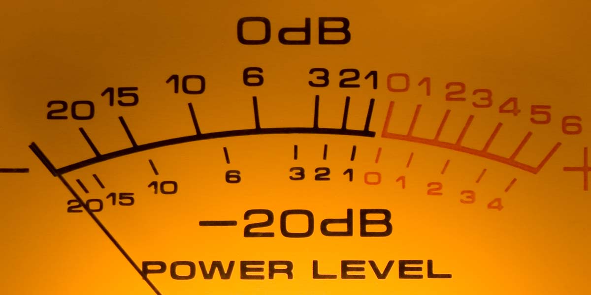
You don’t necessarily have to have a calculator at the ready. Just memorizing the few power dB relationships in Table 1 is easy.
| P2/P1 | dB | V2/V1 | dB |
| 0.1 | -10 | 0.1 | -20 |
| 0.25 | -6 | 0.25 | -12 |
| 0.5 | -3 | 0.5 | -6 |
| 1 | 0 | 1 | 0 |
| 2 | 3 | 2 | 6 |
| 4 | 6 | 4 | 12 |
| 5 | 7 | 5 | 14 |
| 10 | 10 | 10 | 20 |
Table 1 — Decibel Values for Common Power and Voltage Ratios.
Remembering a simple rule for factors of 10 will come in quite handy, too. Speaking in terms of power, any change by an exponent of 10 is a change in dB of 10 times the exponent. A change of 100 (102) is a change of 20 (2 x 10) dB; a change of 1000 (103) is a change of 30 (3 x 10) dB; and so forth.
Another handy thing to remember is that multiplying the ratio by a factor allows you to add the dB equivalent of that factor. For example, from Table 1, a change of 20 is the same as a change of 5 x 4, so a change of 20 in dB is equal to 7 + 6 = 13 dB. You could also figure that out from 20 = 10 x 2, so the dB equivalent is 10 + 3 = 13 dB. Doubling power — another common situation — is a change of 3 dB. By memorizing a few values and rules, you can navigate dB quite easily!
Decibel-defined Values (dBm, dBW, dBV, dBuV)
It’s quite common to need an “absolute” power level, yet need to work with gain and attenuation in dB. The solution is to use a single fixed reference level for all measurements. The value for P1 in the equation shown (the one in the denominator) is the ratio’s reference level. By using the same absolute reference value for all of your calculations, you also know the absolute power of the measurement.
For example, if you use one milliwatt (1 mW) as your reference level, all of your dB values will be calculated “with respect to one milliwatt.” This is so common in wireless that the abbreviation dBm was created. A power level of 10 dBm is 10 times 1 mW or 10 mW; 3 dBm is 2 mW; -20 dBm is 0.01 mW; and so forth. Because values in dB are added or subtracted when the quantities are multiplied or divided, you can easily use dBm values throughout your radio system.
For example, when a 1W transmitter signal (30 dBm) is amplified with a gain of 15 dB, it becomes a 30 + 15 = 45 dBm signal. A received signal of -47 dBm experiencing a cable loss of 6.2 dB is reduced to -47 – 6.2 = -53.2 dBm.
Other common abbreviations you’ll encounter in the wireless world are the dBW (reference level of one watt), dBV (reference level of one volt), and dBuV (reference level of 1 μV). When you see a letter appended to “dB,” it is specifying a common reference value.
Signal-to-Noise Ratio
Another common measurement expressed in dB is the signal-to-noise ratio, or SNR or S/N. SNR compares the signal power to the power of the background noise: SNR = 10 log10 (PSIGNAL / PNOISE). Often left out of the discussion is the bandwidth of the channel over which noise is measured.
For example, a telephony circuit (mobile or landline) may be assumed to have a communications-quality bandwidth of 3 kHz. It’s usually assumed to be the receiver or amplifier bandwidth, but don’t assume that’s always the case. If you really need to know SNR with full accuracy, specify the bandwidth of the measurement.
In the case where interfering signals are also present — such as for a data link in a shared unlicensed frequency band like 900 MHz or 2.4 GHz — a better measurement might be signal-to-noise plus interference ratio or SNIR. (This measurement is also written as signal-to-interference plus noise ratio, or SINR.) If your data link will be operating in a crowded band, this might be a better way to measure and plan your communications link.
Finally, each step in the modulation/demodulation and signal amplification chain adds some distortion products to the desired signal. The measurement signal-to-noise plus interference and distortion, or SINAD accounts for these effects: SINAD = 10 log10 [(PSIGNAL + PNOISE + PDIST) / (PNOISE + PDIST)].
Gain: Power or Pattern
I have mentioned “gain” several times so far in this column and it’s time to explain there are two common definitions, both specified in dB. The most used definition and probably the one you imagine when you see the word is power gain. This is what happens when an active device such as an op-amp or transistor or vacuum tube uses a low level input signal to control a more powerful output signal. The output signal has more power than the input signal. That input-to-output power ratio is the gain of the circuit or device — pretty straightforward.
The other type of gain is created by antenna designers. You’ll frequently see antennas specified to have some value of gain in dB. The antennas themselves do not add any power to the signal applied to their feed point. In fact, due to resistance, the antenna has a slight loss. The gain being referred to — pattern gain — comes from focusing the signal in a certain direction so that it appears stronger in the favored direction. This is equivalent to having amplified the signal by the same amount.
An antenna’s pattern gain, however, is always measured or specified with respect to some standard reference antenna. The two most common references are the isotropic antenna which radiates equally in all three-dimensional directions, and the dipole which radiates best broadside to the antenna and very weakly off the ends.
If you imagine the isotropic antenna’s radiation pattern as a spherical balloon filled with radiated power, a directional antenna like a beam or dish creates pattern gain by “squeezing” the sphere. Where the signal is focused, the sphere extends farther from the center than without focusing. The ratio between the focused direction and the original equal-in-all-directions is the antenna’s gain in that direction.
Since the ratio depends on the reference antenna’s pattern, antenna gain must always be specified with respect to the reference antenna. If the reference was an isotropic antenna, the abbreviation dBi is used; dB with respect to an isotropic antenna. If a dipole was used, the abbreviation dBd is used with the understanding that the dipole’s pattern is used where the dipole’s radiation is strongest: broadside to the dipole. In fact, a dipole has a gain of 2.2 dBi, so you can convert dBd to dBi by adding 2.2 dB and vice versa by subtracting dBi. When you see an antenna advertised as having “x dB of gain,” you have to ask, “With respect to what?”
SWR and Return Loss
The notion of standing wave ratio, or SWR was introduced in my January 2016 article. Basically, it is a measure of how much power in a feed line is transferred to the load and how much is reflected back toward the signal source.
Reflections occur because of a mismatch between the load impedance and the feed line’s characteristic impedance. SWR can have a value of 1:1 (no reflection, all power transferred to the load) and ¥ (all power reflected, as at an open- or short-circuit).
Such a wide range (1 to ¥, but not beyond) is okay for the relatively imprecise world of amateur radio and most hobby applications. Typically, if the SWR a transmitter “sees” looking into a feed line is less than 1.5:1, everything works well. Professionals, however, want a more precise measurement at both high and low values of SWR. They use return loss, or RL.
RL is measured in dB as the ratio between power reflected back toward the signal source and the forward power from the source: RL = -10 log (PREFL / PFWD). If PREFL = 0, then RL = ¥ and SWR is 1:1. If PREFL = PFWD, then RL = 0 dB and SWR is ¥. There is a handy online converter for RL and SWR at the Microwaves101 website at www.microwaves101.com/calculators/872-vswr-calculator.
Effective Radiated Power (ERP)
When planning a wireless communications system or broadcast installation, you have to know the strength of the transmitted signal in order to figure out how well it will be received. With so many different factors affecting radiated signal strength, it’s hard to compare “apples to apples.” As a result, the concept of effective radiated power, or ERP was devised. ERP accounts for gains and losses throughout the entire antenna system, from the transmitter to the antenna. The resulting value represents how much power it would take to create the same signal strength using a standard reference antenna.
The standard antenna can be an isotropic antenna with no pattern gain in any direction or a dipole antenna which has 2.2 dB more gain broadside to the antenna than an isotropic antenna. Like the decibel-defined value discussed earlier, a letter can be added to ERP to indicate which reference is used. EIRP is the ERP calculated with respect to an isotropic antenna; if no letter is added (ERP), then a dipole is assumed to be the reference. To convert ERP to EIRP, add 2.2 dB to account for the dipole’s higher gain.
An example is useful in explaining how ERP works. Figure 1 shows a typical transmitting installation that might be installed at a shared communications site.
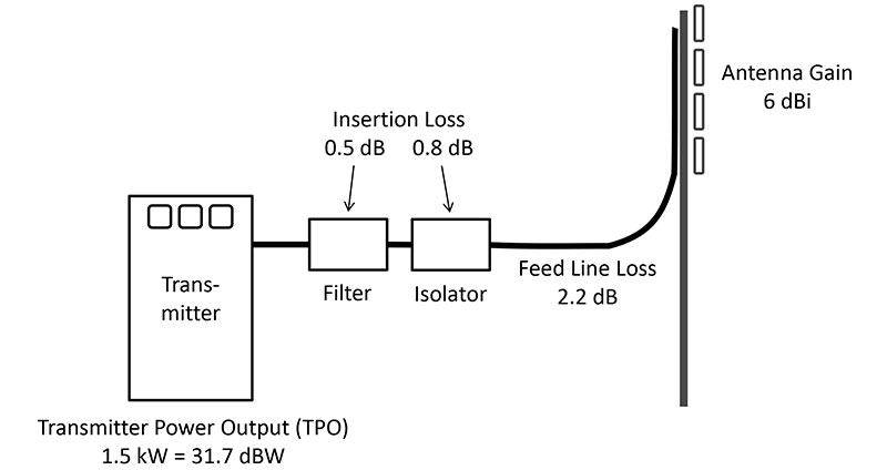
Figure 1.
Let’s start with the transmitter power output, or TPO of 1.5 kW. This is an absolute power level of 10 log10 (1500) = 31.7 dBW. The transmitter is connected to a filter that removes any harmonics but also has an insertion loss, or IL of 0.5 dB. (This loss is due to losses in the inductors and capacitors and connecting wires.)
To prevent other transmitted signals from coming down the feed line and getting into our transmitter output, an isolator is used that only allows power to flow toward the antenna. It, too, has insertion loss, and the amount of loss is 0.8 dB. Feed lines also have loss, and at the frequency of the transmitted signal (for this length of feed line) the loss is 2.5 dB. Finally, the antenna is a bay of folded dipoles with a pattern gain of 6 dBi. So, what is our EIRP and ERP?
- EIRP = TPO – Filter IL – Isolator IL – Feed Line IL + Antenna Gain
- EIRP = 31.5 dBW – 0.5 dB – 0.8 dB – 3.5 dB + 6 dBi = 32.7 dBW = 1862W
- ERP = EIRP – 2.2 dB = 32.7 dBW – 2.2 dB = 30.5 dBW = 1122W
This makes sense because our transmitter would have to work 2.2 dB harder to create the same signal strength at the receiver if it only used an isotropic antenna. As you can see, it’s quite easy to work with dBW and dB instead of having to calculate everything in watts.
Bandwidth and Spurious Emissions
Finally, interference is a fact of life with wireless systems. Sometimes it’s accidental, but it’s always annoying. The FCC (Federal Communications Commission) sets standards for how transmitters must behave in order to be good neighbors and share spectrum. Key to establishing common ground is a clear definition of terms, and one of the most important is bandwidth.
While there are lots of different definitions of bandwidth floating around, there’s only one that matters on the air and that is the FCC’s definition! For the amateur service, bandwidth is defined in the FCC’s rules, Part 97.3(8): The width of a frequency band outside of which the mean power of the transmitted signal is attenuated at least 26 dB below the mean power of the transmitted signal within the band.
What that means is for whatever signal you are transmitting — data, AM voice, FM voice — the FCC will average (take the mean of) the transmitted signal power and find the frequencies on either side of the signal at which the signal’s strength is 400 times (26 dB = 20 dB + 3 + 3 dB = 100 x 2 x 2 = 400) weaker. The difference between those two frequencies is the signal’s bandwidth. Figure 2 gives you an idea of how this works.
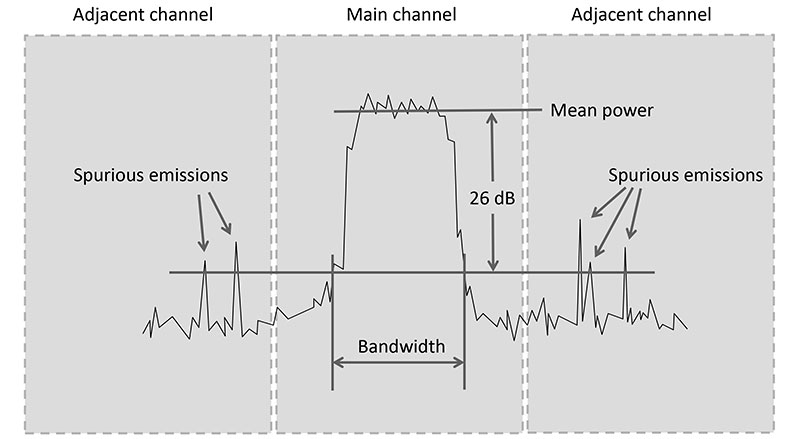
Figure 2.
Spurious emission is the term for any component of the transmitted signal that is unnecessary or unintentional, and which is stronger than 26 dB below the signal’s mean power. As you can see from the figure, spurious emissions far from the signal can cause interference to signals on adjacent channels and, in fact, this is quite common. Perhaps the transmitter is overmodulated, causing extra sidebands to appear to either side.
Perhaps a speech processing circuit isn’t operating properly and distorts the signal and creates these extra signals. Harmonics of a signal are also spurious emissions. These are almost always present because no transmitter is perfect.
There are always some minor non-linearities that produce harmonics. If you have an AM broadcast station nearby with a frequency below 800 kHz, set your car or portable radio to twice the station’s frequency and drive toward the transmitter. At some point, you’ll hear a distorted version of the same programming from the second harmonic of the transmitted fundamental. (There is no “first” harmonic — that’s the fundamental.)
If you have a general-coverage short-wave or “world band” receiver, you can probably find the third harmonic as well. Don’t get too close to the transmitter or your receiver will be overloaded and start generating harmonics internally all by itself! “Spurs” aren’t always the fault of the transmitter!
Signing Off
Decibels are everywhere in wireless communications. They allow us to compare and discuss signals many orders of magnitudes different in amplitude without having to use cumbersome notation or lots of zeroes! Getting comfortable with the “dee-bee” is a great first step in understanding radio signals and the systems that produce them.
Online Glossary
The ARRL’s Technical Portal (arrl.org/tech-portal) includes several references, and you’ll also find an online glossary (www.arrl.org/ham-radio-glossary) that explains terms as hams use and understand them. If you are studying for your ham radio license, these would be good websites to bookmark in your browser.
Noise in Analog-to-Digital Converters (ADCs)
It’s the norm these days to digitize analog signals and manipulate them in software. As such, it’s important to understand the noise performance of ADCs. The Analog Devices’ tutorial — “Understand SINAD, ENOB, SNR, THD, THD + N, and SFDR So You Don’t Get Lost in the Noise Floor” (AD MT-003) — is an excellent tutorial on different noise metrics of ADCs.
You can download it for free at https://www.analog.com/media/en/training-seminars/tutorials/MT-003.pdf